How to use R?
The RStudio window has multiple panes. RStudio IDE Cheat Sheet:
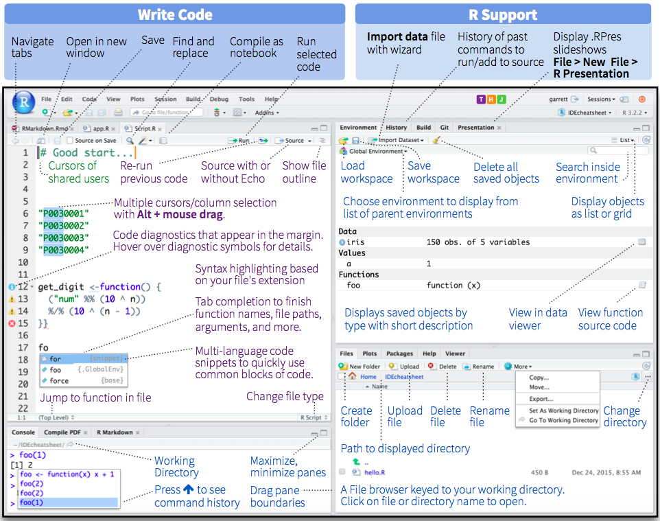
Top Left - Code Editor: for creating scripts to run in pieces or as a whole (like this document!);
Bottom Left - R Console: you can type R commands and see output;
Top Right - Environment: lists the objects that you create, such as data sets;
Bottom Right - Help: find out information about functions and packages. This same pane will have tabs for showing plots that you make, view apps and documents, show files in the folder, and packages used.
R is a scripting language, which means that it is just like writing an essay, or a maths proof. We write a script to do specific tasks, that we can run again and again, or give to someone else to run.
You should take note of the following facts:
- R is a case-sensitive language which executes instructions directly
- Commands are entered at prompt
> - Commands are separate statements which could be put in the same line if separated by a semi-colon
; - Code statements can be commented by using a
#tag. You can comment in continuation of the command line or in a separate line
💡 The best way to learn is by doing. Therefore, I would like you not to copy paste the commands shown in the black boxes, but to type it in your R console. It would be even better to type it as an R script, so that you can keep a history of it and return to it if you wish.
Let’s start using R!
- Turn on your computer (if you haven’t already)
- Open RStudio
- Create a project for your work. On the very right side of the window is a small blue R, and a drop-down menu. Select
New project, thenNew directory, navigate to the desktop, and name the projectMy_First_R. This will create a folder with this name on the desktop. This will be your workspace for this project. 😇
Setting up your working directory
If you want to read or write files on your computer from and to a specific location you will need to set a working directory in R. To set the working directory in R to a specific folder on your computer you will use the following:
# On a pc, you would set the working directory like this
setwd("C:/Documents/MyR_Project")

# On a mac, you would set the working directory like this
setwd("~/documents/MyR_Project")
🤓💡: Make sure you fully adopt the correct syntax in terms of slashes and quotation marks.
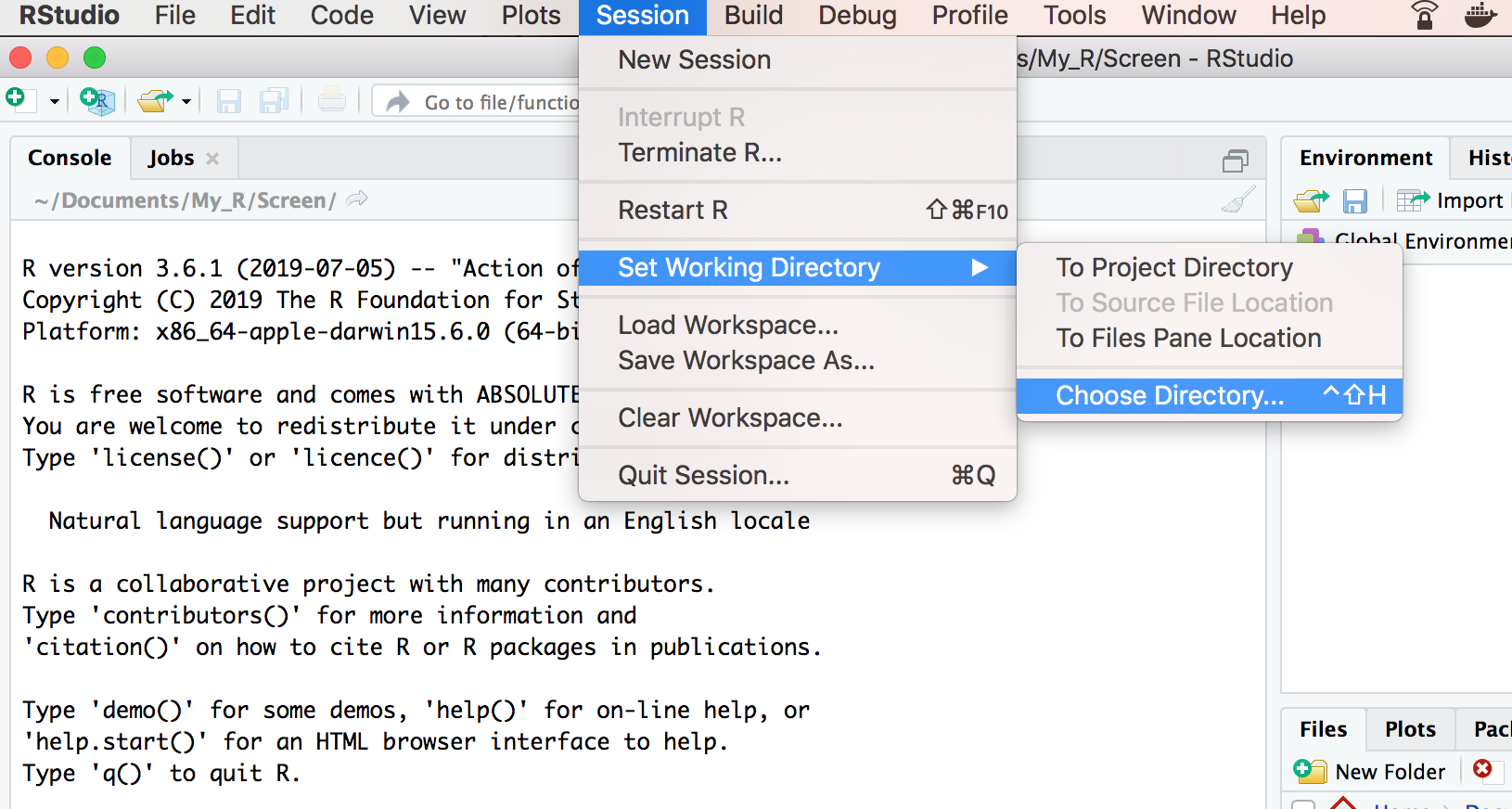
Note that the current working directory is displayed by RStudio within the title region of the Console. You can also set up your working directory by:
- selecting the options available from RStudio’s main menu
Use the Tools | Change Working Dir… menu (Session | Set Working Directory on a mac).
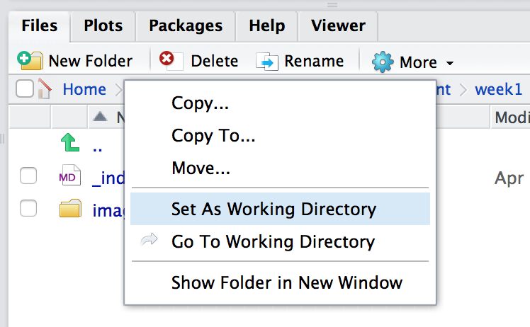
- selecting the option from within the Files pane
Use the More | Set As Working Directory menu
However, you should always start a fresh project (File | New Project…) that will automatically set up your working directory without having to point to it in your script file. You should read the Project-oriented workflow 💻🔥 article by Jenny Bryan to convince yourself that this would be a good habit you should adopt.
R Packages
“In R, the fundamental unit of shareable code is the package." Hadley Wickham, R packages
R packages are collections of functions code, data sets, documentation and tests developed by the community, that are mostly made available on the Comprehensive R Archive Network, or CRAN, the public clearing house for R packages. These packages are developed by experts in their fields and currently the CRAN package repository features over 14,000 of them. Many of the analyses that they offer are not even available in any of the standard data analysis software packages, which is one of the reasons that R is so successful.
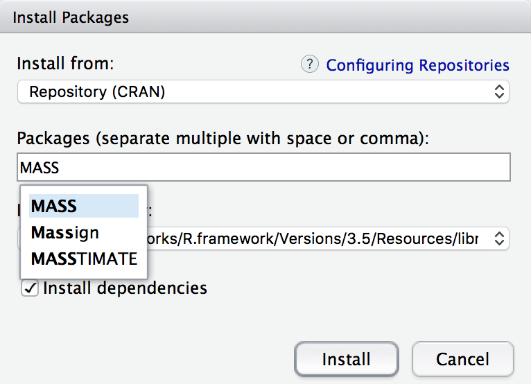
When you run R you will automatically upload the package:base, which is the system library, i.e. the package where all standard functions are defined. The rest of the so called base packages contain the basic statistical routines. Assuming that you are connected to the internet, you can install a package using install.packages(). From the RStudio menu, you can do it by selecting Tools | Install Packages… and typing the name of the desired package in the dialogue window.
Once installed, the package will appear in the list of available packages in your Packages pane. To use it you have to load it to the system’s search path by simply typing the name of the package as an argument of the library() function, or by checking the box next to its name from the Packages pane.
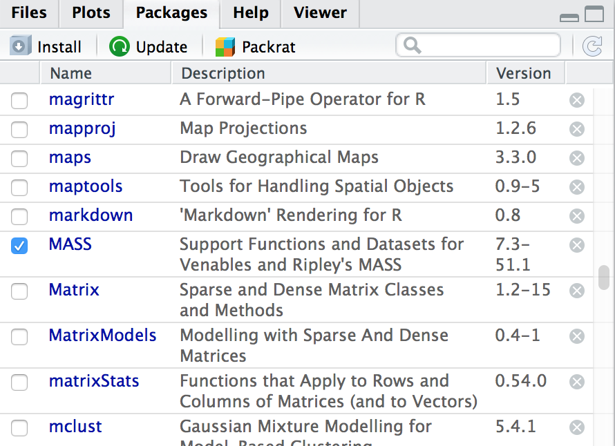
💡: Note that you can call the dialogue window to install a package from Packages pane! Have you spotted the Install icon yet?
Calculate in R
To begin with, we can use R as a calculator. 😁
In your console type in 2 + 2. Note that you don’t have to type the equals sign and that the answer has [1] in front. The [1] indicates that there is only one number in the answer. If the answer contains more than one number it uses numbering like this to indicate where in the ‘group’ of numbers each one is.
You see?! R is like a big calculator! 😲
Arithmetic and Logical Operators
R’s binary and logical operators will look very familiar to those who have some experience with programming.
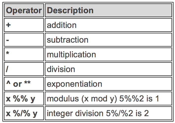
Arithmetic Operators
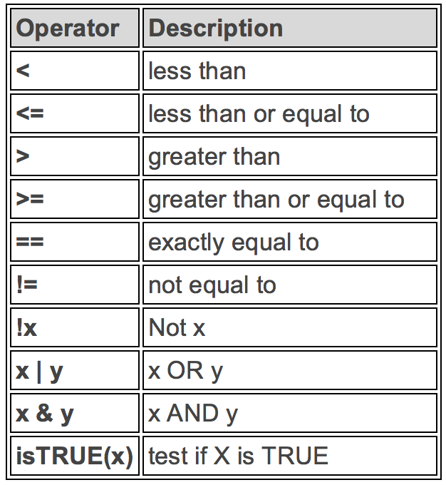
Logical Operators
Try doing other maths operations, like subtraction, multiplication, division, or square root and power operations. For example, try the following:
2 + 5
3 - 2
18 / 6
4 * 7
(5 - 3)^2 / 4
9^(1/2) * 4
Reproducibility: Save your scripts
The code you type and want to be executed can be saved in scripts and R Markdown files. Scripts ending with .R file extension and R Markdown files, which mixes both R code and Markdown code, end with .Rmd.
🤓💡: The code that you write just for quick exploration can be written in the console. Code we want to reuse and show off later should be saved as a script.
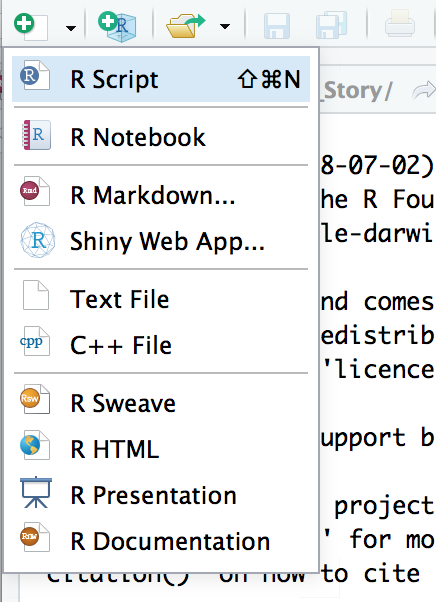
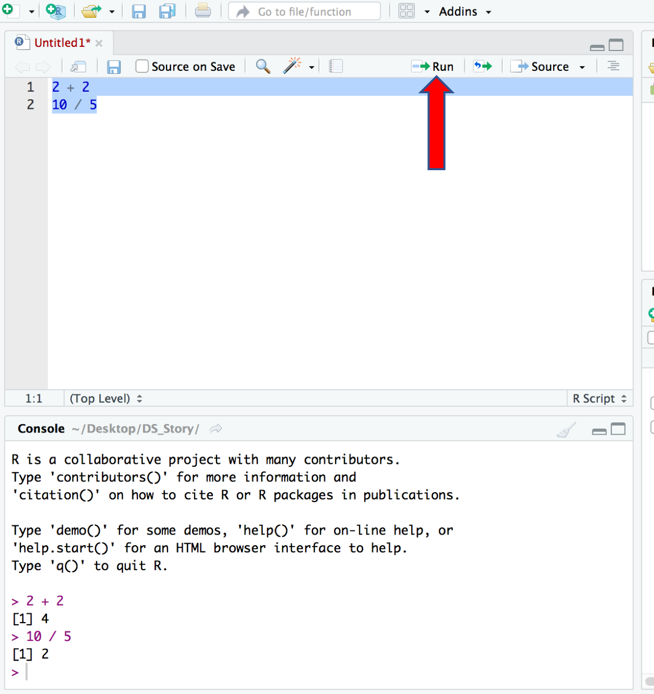
To create a new script go through the menu File | New File | R Script or through the green plus button on the top left.
Any code we type in here can be run and executed in the console. Hitting the Run button at the top of the script window will run the line of code on which the cursor is sitting.
To run multiple lines of code, highlight them and click Run.
💡: Get into the habit of saving your scripts after you create them. Try to save them before running your code in case you write code that makes R crash which sometimes happens. 😣 &@#$!?#%
https://www.rstudio.com/products/rstudio/features/
R Objects
R provides a number of specialised data structures we will refer to as objects. To refer to an object we use a symbol. You can assign any object using the assignment operator <-, which is a composite made up from ‘less than’ and ‘minus’, with no space between them! Thus, we can create scalar constants, which we refer to as variables, and perform mathematical operations over them.
x <- 5
y <- 6
You can use objects in calculation in exactly the same way as you have already seen numbers being used earlier:
x + y
and you can store the results of the calculation done with the objects in another object:
z <- x * y
z
🤓💡 BUT, remember!!! Operator <- is a composite made up from ‘less than’ and ‘minus’, with no space between them!!!!
Try to type the following
x< -5
y< -6
and see what happens.
After you’ve created some objects in R you can get a list of them using ls() function:
ls()
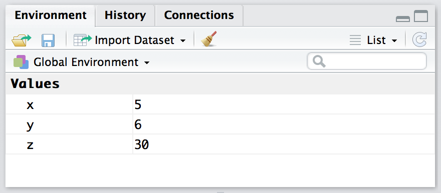
RStudio provides a very comfortable working environment and enables you to monitor your list of objects in the Environment pane window in the top right corner.
Built-In Functions
R is not like other conventional statistical packages like SAS, Minitab, SPSS, to name a few. It is more of a programming language designed for conducting data analysis. It comes with a vast number of ready-made blocks of code that will enable you to manipulate data, perform intricate mathematical calculations with data, carry out an array of statistical analyses ranging from simple to complex to extremely complex and it will facilitate the creation of fantastic graphs. These pre-made blocks of code are known as functions.
R has all the standard mathematical functions that you might ever need: sin, cos, tan, asin, atan, log, log10, exp, abs, sqrt, factorial… To use them, all you need to do is to type the function and put the name of the object (argument) you would like to use the function for in brackets.
You should try a few 😃
sqrt(144)
log10(8)
log10(100)
log(100)
exp(1)
pi
sin(pi/2)
abs(-7)
factorial(3)
exp(x)
log(y, 2)
You can use expression as the argument of a function:
z <- x * y
trunc(x^2 + z / y)
log((100 * x - y^2) / z)
You can have nested functions and you can use functions in creating new objects:
round(exp(x), 2)
p <- abs(floor(log((100*x - y^2) / exp(z))))
p
🤓💡 To obtain a description of a function you need to type a question mark, ?, in front of the name of the function. You might find this particularly useful when you start applying more complicated functions, as help will often provide you not only with the detailed description of the function’s input/output arguments, but practical illustrative examples on how the function can be used and applied. You should try to ask R for help for lm() function (can you tell what it is used for?)
Vectors
When analysing data you are more likely to be working with lots of numbers/variables. It would be much more convenient to keep all of those numbers/variables as an object. Variables can be of different types: logical, integer, double, string are some examples. Variables with one or more values of the same type are vectors. Hence, a variable with a single value (known to us as a scalar) is a vector of length 1. We can assign to vectors in many different ways:
- generated by R using the colon symbol (
:) as a sequence generated operator or by using the built in functionrep()for replicating the given number for a given number of times.
x <- 1:10
x
## [1] 1 2 3 4 5 6 7 8 9 10
x <- rep(1,10)
x
## [1] 1 1 1 1 1 1 1 1 1 1
- generated by the user by using concatenation function c that allows you to enter one number at a time
x <- c(2, 6, 4, 2, 3, 7, 1, 5, 9, 8)
x
## [1] 2 6 4 2 3 7 1 5 9 8
- created as a sequence of numbers. For example to generate a sequence of numbers from 1 to 10, with increments of 0.2 type
seq(1,10,0.2)
##  [1]  1.0  1.2  1.4  1.6  1.8  2.0  2.2  2.4  2.6  2.8  3.0  3.2  3.4  3.6  3.8
## [16]  4.0  4.2  4.4  4.6  4.8  5.0  5.2  5.4  5.6  5.8  6.0  6.2  6.4  6.6  6.8
## [31]  7.0  7.2  7.4  7.6  7.8  8.0  8.2  8.4  8.6  8.8  9.0  9.2  9.4  9.6  9.8
## [46] 10.0
💡: R can easily perform arithmetic with vectors as it does with scalars. Thus, just as we can use these operators over scalars we can use them when dealing with vectors and/or a combination of both.
x <- rep(1,10)
y <- 1:10
x
## [1] 1 1 1 1 1 1 1 1 1 1
y
## [1] 1 2 3 4 5 6 7 8 9 10
c(x, y)
## [1] 1 1 1 1 1 1 1 1 1 1 1 2 3 4 5 6 7 8 9 10
x + y
## [1] 2 3 4 5 6 7 8 9 10 11
x + 2 * y
## [1] 3 5 7 9 11 13 15 17 19 21
x^2 / y
##  [1] 1.0000000 0.5000000 0.3333333 0.2500000 0.2000000 0.1666667 0.1428571
##  [8] 0.1250000 0.1111111 0.1000000
z <- (x+y)/2
z
## [1] 1.0 1.5 2.0 2.5 3.0 3.5 4.0 4.5 5.0 5.5
z <- c(z, rep(1, 3), c(100, 200, 300))+1
z
##  [1]   2.0   2.5   3.0   3.5   4.0   4.5   5.0   5.5   6.0   6.5   2.0   2.0
## [13]   2.0 101.0 201.0 301.0
p <- 2.5
z*p
##  [1]   5.00   6.25   7.50   8.75  10.00  11.25  12.50  13.75  15.00  16.25
## [11]   5.00   5.00   5.00 252.50 502.50 752.50
Accessing A Vector’s Elements
To access a specific element of a vector you would use index inside a single square bracket [] operator. The following shows how to obtain a vector member. The vector index is 1-based, thus use index position 4 to access the fourth element.
x <- c(9, 3, 7, 2, 9, 2, 1, 5, 4, 6)
x
## [1] 9 3 7 2 9 2 1 5 4 6
x[4]
## [1] 2
💡: In R you can evaluate functions over the entire vector which helps to avoid looping.
y <- c(4, 1, 0, 8, 1, x)
max(y)
## [1] 9
range(y)
## [1] 0 9
mean(y)
## [1] 4.133333
var(y)
## [1] 9.409524
sort(y)
## [1] 0 1 1 1 2 2 3 4 4 5 6 7 8 9 9
cumsum(y)
## [1] 4 5 5 13 14 23 26 33 35 44 46 47 52 56 62
💡: Note that missing values in R are represented by the symbol NA (not available) or NaN (not a number) for undefined mathematical operations.
Here, NA would be shown if an index is out-of-range.
z <- c(5, 8, 2)
z[10]
## [1] NA
You can also obtain a desirable selection of the elements of a vector by specifying a query within the index brackets []:
y <- c(9, 3, 7, 2, 9, 2, 1, 5, 4, 6)
y[y > 5]
## [1] 9 7 9 6
y[y > 10]
## numeric(0)
y[y != 2]
## [1] 9 3 7 9 1 5 4 6
Matrices
When data is arranged in two dimensions rather than one we have matrices. In R function matrix() creates matrices:
ma1 <- matrix(c(1, 0, -20, 0, 1, -15, 1, -1, 0),
              nrow = 3, ncol = 3,
              byrow = TRUE)
ma1
##      [,1] [,2] [,3]
## [1,]    1    0  -20
## [2,]    0    1  -15
## [3,]    1   -1    0
dim(ma1)
## [1] 3 3
The individual numbers in a matrix are called the elements of the matrix. Each element is uniquely defined by its particular row number and column number. To determine the dimensions of a matrix use function dim().
An element at the i-th row, j-th column of a matrix can be accessed by indexing inside square bracket operator [i, j]. The entire i-th row or entire j-th column of a matrix can be extracted as shown in the code below.
ma1 <- matrix(c(4, 10, 130, 0, 8, -7, 9, 11, -2, 7, -5, 4),
              nrow = 3, ncol = 4)
ma1
##      [,1] [,2] [,3] [,4]
## [1,]    4    0    9    7
## [2,]   10    8   11   -5
## [3,]  130   -7   -2    4
ma1[2, 3]
## [1] 11
ma1[1, ]
## [1] 4 0 9 7
ma1[ , 4]
## [1] 7 -5 4
Standard scalar algebra, which deals with operations on single numbers, has a set of well established rules for handling manipulations involving addition, subtraction, multiplication and division. In a broadly similar fashion, a set of rules has been developed to enable us to manipulate matrices. However, introducing those rules is beyond the scope of this course, but they are nicely covered on the www.statisticshowto.com website.
YOUR TURN 👇
Practise by doing the following set of exercises:
-
Create vectors called
x1andx2, where vectorx1consists of numbers:1, 4, 7, 9, 11, 12, 13, 15and18and vectorx2of numbers:1, 1, 1, 2, 2, 2, 3, 3, 3. -
Subtract
x2fromx1. -
Create a new vector called
x3by combining vectorsx1andx2. -
Calculate mean and variance of
x3. -
Calculate medians for the three vectors.
-
Create a matrix called
m1with the following elements:matrix(c(1, 5, 9, 2, 6, 10, 3, 7, 11, 4, 8, 12), nrow = 4, ncol = 3, byrow = TRUE) -
Use a subscript to find the
2-nd number in vectorx1andx2and the element in the2-nd row and3-rd column in matrixm1. -
Add the
5-th number in vectorx1to the element in matrixm1which is in1-st row and1-st column. -
Calculate the mean of all numbers in
x3that are less than 13.
Material is released under a Creative Commons Attribution-ShareAlike 4.0 International License.